For a graduate neuronal networks class I took last semester at NYU, I had a project of trying to implement some kind of neuronal network. Given my interest in clustering, I sought to replicate Martí and Rinzel's (2013) feature categorization/clustering network.

Here I show an in-browser demo of their clustering network, as well as a small modification I made to it for anomaly detection. It's kind of fun to play around with (click here to jump directly to it). Most of the parameters in Martí and Rinzel's paper can be modified here to see what effects they have.

The network is an example of a continuous attractor network, which is to say that instead of imagining discrete cells connected to each other, you have an infinite number of cells connected to each other. In some sense, the math becomes easier because you use an integral instead of a sum. However, in this JavaScript demo, I use discrete cells (which can be increased to however many you like, it just makes the simulation slower).

Cells in this network are connected in a ring, and you can imagine each cell as being sensitive to a particular orientation in a line, just like certain visual neurons respond to particular orientations. What this network is going to try to cluster is different orientations that are input into it over time. For example, if the network sees a bunch of nearly flat lines (around $\theta = 0$) over a short period of time, the cells around $\theta = 0$ will begin to maintain a high firing rate. If only a few flat lines are presented though, the cells will forget it and not form a "cluster".

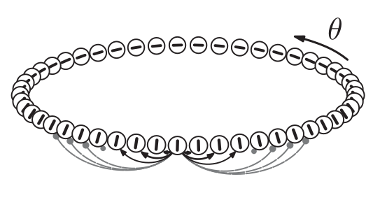
Nearby cells in the ring are connected to each other. With neighboring cells tending to excite each other, slightly further cells tending to inhibit each other, and even further cells having almost no influence. The general shape of the connectivity kernel is what's called a Mexican hat (here approximated with a difference of Gaussians). The general form of this kernel is

\begin{align} J(\theta) &= J_E(\theta) - J_I(\theta)\\ &= j_E \frac{\exp\left(m_E \cos(2\theta)\right)}{I_0(m_E)} - j_I \frac{\exp\left(m_I \cos(2\theta)\right)}{I_0(m_I)} \end{align}

where "$E$" is for excitation and "$I$" inhibition, with $m$ changing the narrowness and $j$ the height of the Mexican hat. "$\theta$" here is the angle difference between neighboring cells. You can mess around with the parameters in the "Kernel" section below to see the effect of different values.

There are two variables that we simulate over time, $s(\theta, t)$, which is the synaptic activation, and $r(\theta, t)$, which represents cell firing. For anomaly detection, I add a third variable $y(\theta, t)$. \begin{align} \tau \frac{\partial}{\partial t}s(\theta, t) &= -s(\theta, t) + r(\theta, t)\\ r(\theta, t) &= \Phi \left[ \frac{1}{\pi} \int_{-\pi/2}^{\pi/2} J(\theta - \theta')s(\theta', t) d\theta' + I(\theta, t)\right]\\ y(\theta, t) &= \Phi(I(\theta, t)) * (1 - s(\theta, t)) \end{align}

Here, $\Phi(x)$ is a sigmoid function for converting a current to a firing rate (between 0 and 1). Its equation is \begin{align} \Phi(x) &= \frac{1}{1 + exp(-\beta[x - x_0])} \end{align} and can be modified in the "Current-to-Rate" section.

The third section, "Excitation", describes how cells respond to stimuli. This basically shows how sensitive cells are to nearby orientations. It has two parameters, $m_s$ and $I_s$ that determine narrowness and the amount of current a cell receives to a nearby orientation. You can modify the inputs to the network by clicking directly on the graph to add more input points. Modifying the "Excitation" section changes how wide and strong each click input is.

Other parameters that can be modified include the length and number of time steps, the number of cells simulated in the network, and the time constant $\tau$.

On the x-axis of the graphs below is time. The y-axis ranges from $-\pi/2$ to $\pi/2$, and represents the orientation of different cells in the network.

This network's fairly interesting. Given the right settings it can detect a number of different clusters of different sizes. With the "anomaly detector" addition, we use the cluster detection to suppress non-novel stimuli. A couple potential problems with this network, though, are that clusters can possibly drift over time and will stay activated indefinitely (which may be problematic for anomaly detection).

Run Stop Clear inputs Example Inputs

Recently I had an MRI done on me as part of an MRI scanner operator training session. I decided to hold a face for the T1 scan, which is actually quite difficult because the process takes 5 minutes. Muscles in your face, I believe, aren't supposed to hold the same expression for several minutes in a row, and if you ever try it you'll find your face muscles twitching quite a bit.

I got a copy of my scan and used AFNI and Blender to render the voxel data as I described in an earlier post. I can't decide if the result is creepy or funny looking, haha.

In my last post I talked about using Blender to render MRI volumes. This had the benefit of creating fairly nice static images or movies. In an earlier post I also showed how to use XTK to render volumes in real time.¹ In this post I'll show a similar method of rendering a brain volume in real time using three.js, a Javascript library providing facilities for WebGL.

This process is relatively straightforward. Using these steps from my last post you can get a Wavefront OBJ file from an MRI volume. This object file will have a very large number of polygons, which may make loading and rendering the object in WebGL slower. In order to reduce the number of polygons, import the Object file into Blender and apply the decimate modifier on each hemisphere. Then export the hemispheres as an OBJ file. My resulting OBJ file is linked here.

Then we can basically just modify the object loader three.js example to load our brain!

I outside of the normal minified three.js library I have one main script that handles the interactive rotation and placement of the WebGL container and I've slightly modified the OBJLoader.js script to compute vertex normals (geom.computeVertexNormals();), making the brain appear smoother.

Footnotes:

1. XTK can actually handle FreeSurfer meshes, so using three.js isn't strictly necessary.

In one of my posts I talked about using rendering brain volumes in-browser using XTK. The results, I’ll admit, weren’t spectacular. The volume rendering didn’t really give very defined edges. But now I’ll show a couple methods of rendering a brain using Blender. The first method is using volumetric data in Blender, and the second uses surfaces generated by FreeSurfer. I think it gives pretty cool results, check it out below.

Read More