In a couple of my previous posts I talked about using clustering colors with k-means and counting clusters with EM. This kind of clustering is fairly straightforward, as you have some notion of distance between points to judge similarity. But what if you wanted to cluster text? How do you judge similarity there? (There are certain measures you could use, like the F-measure, which I’ll talk about in a later post.)

One way is to use Latent Dirichlet Allocation, which I first heard about while talking to a Statistics 133 GSI, and then later learned about while reading probabilistic models of cognition. Latent Dirichlet Allocation is a generative model that describes how text documents could be generated probabilistically from a mixture of topics, where each topic has a distribution over words. For each word in a document, a topic is sampled, from which a word is then sampled. This model gives us probabilities of documents, given topic distribution and words. But what’s more interesting here is learning about topics given the observed documents.

Here’s the plate notation view of LDA, which describes exactly how documents are generated:

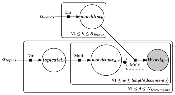
The image above was created using TiKZ-bayesnet (TiKZ is super-fun by the way) for LaTeX, which actually provides an LDA example. I’ve taken their example here and modified the variable names and layout slightly to match my code.

Each box is a “plate” which signifies that the structure should be repeated according to the sequence in the plate’s lower right corner. Think of it like a “for-loop” for graphs.

Now I’ll go over all these variables.

• $alpha_{topics}$ and $alpha_{words}$ are hyperparameters that you set by hand. They show how the Dirichlet distributions create distributions over topics and words, respectively. A Dirichlet distribution outputs a vector that sums to 1, which can be used as the probabilities for a multinomial distribution. We’ll usually set $alpha_{topics}$ and $alpha_{words}$ to be a number greater than 0, but much less than 1. The idea here is that we generate mixtures that are very different from each other. Take a look at the picture below, which represents some sampling from a Dirichlet distribution over 3 categories for different values of the $alpha$ parameter. (Actually $alpha$ is itself a vector of 3 numbers, so $alpha$ of 1 really means $alpha$ is [1, 1, 1])

  

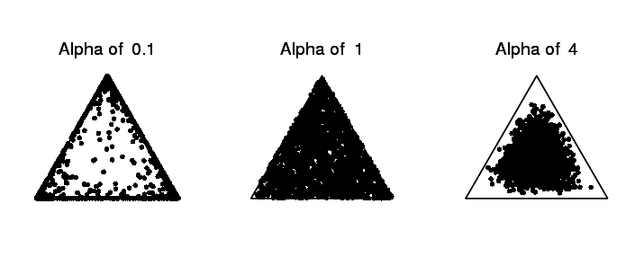
  The leftmost distribution creates highly varied samples. Think of the three points as the proportion of three different words, like “dog”, “cat”, and “mouse”, and we’re generating topics. This might create topics like [8, 0.1, 0.1] (mostly dog), [0.2, 0.9, 0] (mostly cat), etc. Whereas the rightmost distribution creates topics that are much more in the center, which means they’re much closer to each other. Here we might create topics like [0.3, 0.4, 0.3], which means the word “dog”, “cat”, and “mouse” are almost equally likely to be generated by this topic. Smaller alpha values should give much more distinguishing topics, though I would suspect that setting them too small would give unrealistic topics. (e.g. a topic that is only the word “the”)

• $worddist_k$ is a vector as long as the number of unique words we have in all the documents. For each topic $k$, it tells us how frequently a word is generated under that topic.
• $topicdist_d$ is a vector as long as the number of topics we’re modeling. A vector of length $k$ (the number of topics) is generated for each document $d$, which describes “how much” of each topic is represented in a document. If you think documents are usually only ever 1 topic, you’d probably set $alpha_{topics}$ really low. If you think documents contain words from a number of topics, you’d probably set $alpha_{topics}$ slightly higher.
• For each word in a document, we draw a topic $wordtopic_d,w$ from the output of $topicdist_d$. $wordtopic_d,w$ is an integer, like “1” for topic 1.
• $word_d,w$ is observed. It represents the word we actually saw. $word_d,w$ in our model is also an integer like “37” which represents the 37th unique word in our list of words over all documents.

Put all together, the model looks like this in JAGS:

model {
      for (k in 1 : Ktopics ) {
          worddist[k,1:Nwords] ~ ddirch(alphaWords)
      }
      for( d in 1 : Ndocs ) {
           topicdist[d,1:Ktopics] ~ ddirch(alphaTopics)
           for (w in 1 : length[d]) {
               wordtopic[d,w] ~ dcat(topicdist[d,1:Ktopics])
               word[d,w] ~ dcat(worddist[wordtopic[d,w],1:Nwords])
           }
      }
}

Of the four variables here (excluding hyperparameters), three are unobserved, which means the model learns them. I think the most interesting one is $worddist_k$ which will show us what each topic looks like. Here’s an example of what topics might look like visualized as a word cloud. In this example I took the first paragraphs of the “Dog”, “Cat”, and “Mouse” Wikipedia article.

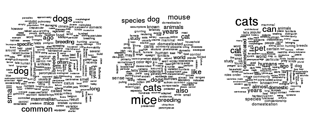
You would hope that the three topics could be separated cleanly—showing mainly “cat” in one topic, “dog” in another, and “mouse”/“mice” in the last—, but I currently haven’t had all that much success with this. This example is also kind of cheating, too, in that maybe for this case I could just do supervised learning with a naive Bayes classifier since I know how all the documents should be clustered.

I initially tried using LDA to cluster different lines from my system log. I later moved to using a dendrogram clustering system using the “F-measure” or “Word Error Rate”, which worked much better both speed and accuracy wise. I may talk about this in a later post.

In the code I’ve included below I also show my failed attempt to detect the number of clusters by fitting multiple models with different numbers of clusters and measuring deviance (something similar to a penalized version of log likelihood, if I understand correctly) to see which fits best. (I may try this with Stan in the future, which will directly give you the log likelihood.) I also show how you can use a library like snowfall to fit multiple JAGS models in parallel. Sampling is embarrassingly parrallel, so there’s no reason to leave your other CPU cores idle while one does all the work.

I think LDA is more interesting when you’re studying topics, instead of trying to simply cluster documents. Ideally I’d like to do more of an unbounded or hierarchical LDA, where the number of topics could vary (or in the case of hierarchical LDA, topics have child topics), but I’ve yet to implement this. What I really liked about the Church programming language was that implementing unbounded models was fairly straightforward. Not so in JAGS. This may be possible to implement in Stan, which would be fun and interesting to do at some point.

Anyhoo, here’s the code: